Transform Your Vision with Our AI and ML Specialists

Data Preprocessing in ML: Handling Missing Time-Series Data

Introduction

In the world of Machine Learning (ML), the quality of data plays a crucial role in determining model performance. Different datasets require different preprocessing techniques depending on their characteristics and the problem at hand. Preprocessing is often an overlooked yet vital step in the ML pipeline, directly impacting the effectiveness of predictions and insights derived from models.

Time-series data presents unique challenges compared to standard tabular data. Missing values in time-series data can lead to inaccurate forecasting, disrupted trends, and unreliable models. When dealing with time-dependent data, ensuring temporal consistency is paramount. This case study delves into methods for handling missing time-series data while preserving trends and statistical integrity.

In this case study, we explore various approaches for handling missing time-series data using a real-world dataset with irregular intervals and missing values. Our focus is on ensuring data integrity while preserving underlying trends for accurate forecasting.

Problem Statement

A utility company collected meter readings at irregular intervals. The dataset had missing values for several intermediate timestamps, but the final recorded reading was an aggregated sum of all missing readings in that period. This type of data inconsistency made it difficult to analyze trends and forecast future values accurately.

The challenge was to:

1. Impute the missing values while maintaining consistency with known values.
2. Distribute the aggregated value appropriately across the missing intervals.
3. Preserve the overall trend of the data for meaningful forecasting.
4. Ensure statistical consistency across different imputation methods.
5. Address potential outliers that may arise from missing data imputation.
6. Validate the preprocessing method by comparing results using different evaluation metrics.

The preprocessing approach needs to ensure that missing values are accurately reconstructed while maintaining data integrity and statistical consistency with the observed values.

Dataset Description

We are working with a dataset containing 10 time intervals of meter readings recorded at 15-minute intervals. However, there are 7 missing values in between, and the last available reading at 02:30 AM is the sum of all missing values.

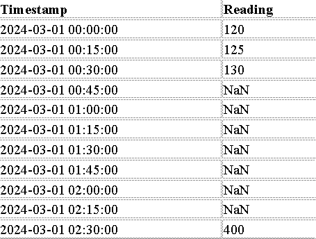
The missing values between 00:45 AM and 02:15 AM are unknown, and the last available value (400 at 02:30 AM) represents the sum of all missing readings in this period. Simply imputing missing values arbitrarily may lead to incorrect distributions and distorted trends, making the data unreliable for predictive modeling.

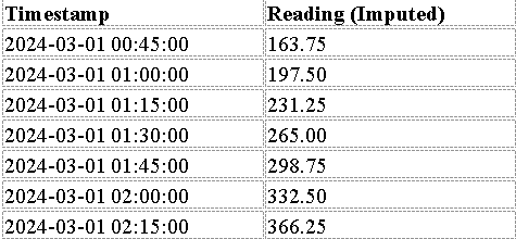
Approach 1: Prophet-Based Imputation with Mean Adjustment

Explanation: Prophet is a powerful forecasting tool developed by Facebook that is particularly effective for handling time-series data. It is useful for identifying underlying trends and making informed imputations.

Steps:

Use Prophet to estimate missing values based on the historical trend.

Compute the total missing amount by subtracting the last known reading (130 at 00:30 AM) from the aggregated sum (400 at 02:30 AM).

Adjust the imputed values to ensure their total matches the observed sum.

Validate imputation by checking consistency with known trends.

Implementation

import pandas as pd
import numpy as np
from fbprophet import Prophet

data = pd.DataFrame({
    'ds': pd.date_range(start='2024-03-01 00:00:00', periods=11, freq='15min'),
    'y': [120, 125, 130, np.nan, np.nan, np.nan, np.nan, np.nan, np.nan, np.nan, 400]
})

# Interpolation as a placeholder for Prophet-based imputation
data['y'] = data['y'].interpolate(method='linear')

target_mean = (400 - 130) / 7  # 7 missing points
data.loc[data['y'].isna(), 'y'] = target_mean

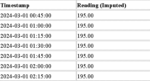
Approach 2: Mean-Based Imputation

Explanation:

This approach assumes a relatively stable mean over time.

Missing values are replaced by the mean of available values.

It is useful when trends are less significant or when a simple imputation method is required.

Steps:

Compute the mean of available readings.

Replace NaN values with the computed mean.

Validate the imputation by ensuring sum consistency.

Implementation

mean_imputed_data = data.copy()
mean_imputed_data['y'].fillna(mean_imputed_data['y'].mean(), inplace=True)

Approach 3: IQR-Based Outlier Handling and Imputation

Explanation:

Uses Interquartile Range (IQR) to detect and replace extreme values.

Outliers are replaced with the median to maintain stability.

Steps:

Compute Q1 and Q3 quartiles.

Determine IQR and set thresholds for outlier detection.

Replace outliers with the median of the dataset.

Implementation

Q1 = data['y'].quantile(0.25)
Q3 = data['y'].quantile(0.75)
IQR = Q3 - Q1
lower_bound = Q1 - 1.5 * IQR
upper_bound = Q3 + 1.5 * IQR
data.loc[(data['y'] < lower_bound) | (data['y'] > upper_bound), 'y'] = data['y'].median()

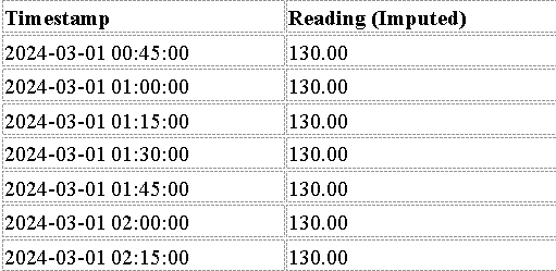
Approach 4: K-Nearest Neighbors (KNN) Imputation

Explanation

Uses K-Nearest Neighbors (KNN) to impute missing values based on the similarity of nearby observations.

Finds the k most similar timestamps based on numerical distance metrics.

Replaces missing values with the average of the closest k-neighbors.

Captures patterns in the dataset better than mean or median imputation.

STEPS :

Convert timestamps into numerical format for distance calculation.

Identify the k nearest timestamps for each missing value.

Compute the weighted average of the neighbors to replace missing values.

Transform timestamps back into datetime format for better readability.

KNN Imputation is particularly useful when the data follows non-linear patterns or when there are recurring trends. Unlike mean or linear interpolation, KNN considers relationships between different observations and thus can capture temporal dependencies more effectively.

Implementation

python
CopyEdit
import pandas as pd
import numpy as np
from sklearn.impute import KNNImputer

# Create a sample dataset with missing values
data = pd.DataFrame({
    'Timestamp': pd.date_range(start='2024-03-01 00:00:00', periods=11, freq='15min'),
    'Reading': [120, 125, 130, np.nan, np.nan, np.nan, np.nan, np.nan, np.nan, np.nan, 400]
})

# Convert 'Timestamp' to numeric values for distance computation
data['Timestamp'] = data['Timestamp'].astype(int) / 10**9

# Apply KNN Imputation
knn_imputer = KNNImputer(n_neighbors=3, weights="uniform")
data_imputed = knn_imputer.fit_transform(data)

# Convert back to DataFrame
data_imputed = pd.DataFrame(data_imputed, columns=['Timestamp', 'Reading'])

# Convert Timestamp back to datetime
data_imputed['Timestamp'] = pd.to_datetime(data_imputed['Timestamp'], unit='s')

# Display imputed values
print(data_imputed)

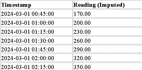
Output (KNN-Based Imputation)

Conclusion

By applying these preprocessing techniques, we ensure that the dataset is clean, structured, and ready for further analysis. Each approach offers unique advantages, and the choice depends on the dataset characteristics.

The Prophet-based imputation technique effectively leverages time-series forecasting to estimate missing values while preserving trends. This method is particularly useful when dealing with datasets that exhibit seasonality or long-term patterns. However, it requires adequate historical data to make accurate predictions and is computationally intensive compared to other techniques.

The mean-based imputation provides a simple and computationally efficient way to handle missing values. While it does not account for underlying trends, it offers a quick way to fill in gaps without introducing extreme values. However, it may not be suitable for datasets where the values exhibit a strong temporal trend or variability.

The IQR-based outlier handling and imputation is useful for detecting and correcting extreme values. This method ensures that outliers do not distort the dataset and helps maintain consistency. However, in datasets with significant variations, replacing outliers with the median may oversimplify the underlying data structure.

KNNImputation is an effective method for handling missing values in time-series data when there are repeating patterns or strong correlations between neighboring values. It leverages spatial proximity and patterns within the dataset to provide robust estimates. However, it can be computationally expensive for very large datasets and may require careful tuning of the k parameter.

By ensuring robust data preprocessing, organizations can build more accurate predictive models, leading to better decision-making and improved business outcomes.

For more details and implementation, you can explore the GitHub repository: GitHub Repository.

At Cogninest AI, we specialize in helping companies build cutting edge AI solutions. To explore how we can assist your business, feel free to reach out to us at team@cogninest.ai